Spins, Magnetism, and Spin-Orbit Coupling ¶

In the original formulation, DFT did not consider electron spin, but extensions to magnetic moments (i.e. spins) were developed quickly after. Like most DFT codes, SIESTA also supports the use of spin components. This tutorial introduces SIESTA calculations with spin and spin-orbit coupling, and how to analyze the results of such calculations.

Specifically, you will learn how to calculate the following physical properties:

the total magnetic moment of a magnetic material
the magnetic moment per atom/orbital
the spin-resolved density of states
the effect of spin-orbit coupling

Contents of this tutorial

Spins, Magnetism, and Spin-Orbit Coupling

First Contact with Spins (10 min)¶

Goal of the exercise

Perform a spin-polarized SIESTA calculation.
Extract the spin magnetic moment from the SIESTA output.

As the first example, you are going to perform calculations for bulk iron (Fe) in a body-centered cubic crystal structure. Due to partially filled $3d$ shells, Fe exhibits a spin magnetic moment.

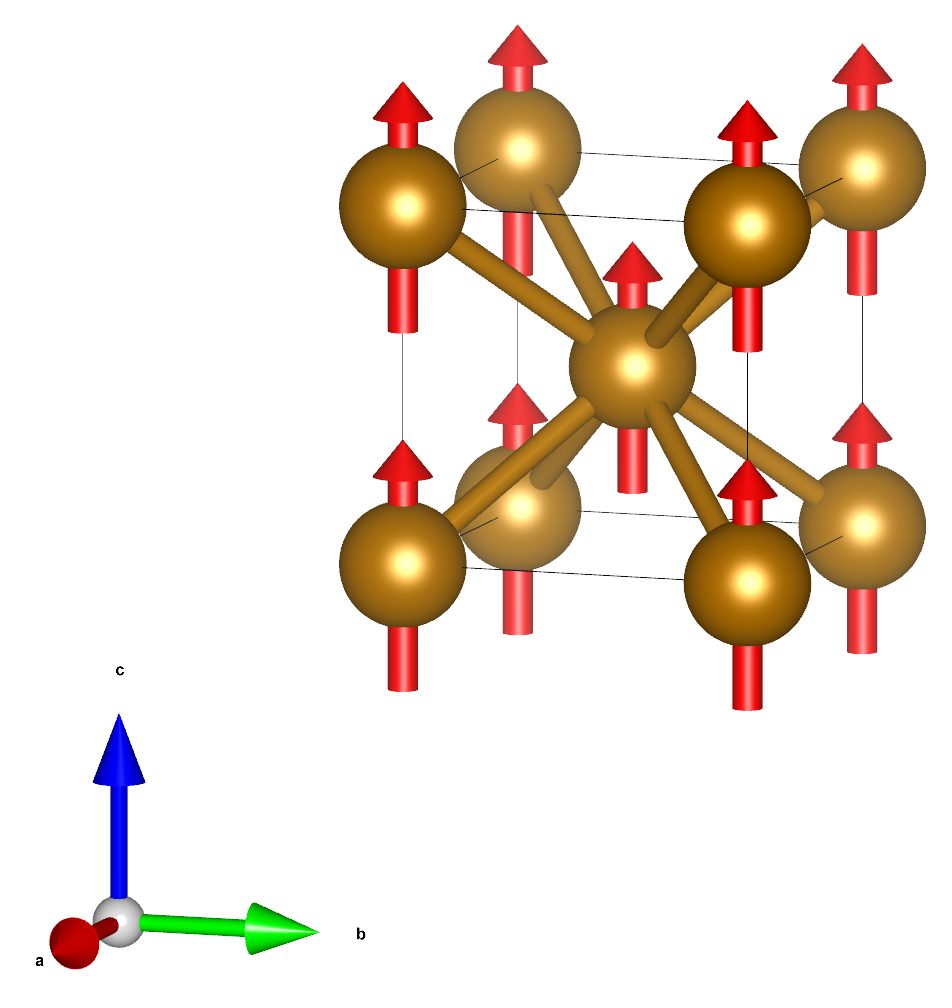
Fig. 11 Ball and stick model of iron (bcc).¶

By default, SIESTA performs calculations without spin. In order to simulate the material with spin polarization, we need to explicitly enable spins in the input files. We can request a spin-polarized calculation by including the line:

Spin polarized

in the input file.

Simulations¶

Hint

Enter the directory ‘01_Fe_bcc’

Take a close look at the input file (fe_bcc.fdf) and familiarize yourself with all the options specified within.
Run SIESTA with and without spins in two separate subfolders. Each calculation should only take a few seconds (about 3 sec on 4 cores).

Analysis¶

Compare the results of the two calculations.

You should see that the SIESTA output contains extra information when running with spins. Specifically, you will find information about the initial magnetic moment (corresponding to the initial guess for the density matrix), the magnetic moment at each SCF step, and the final magnetic moment. Look for lines like this in the output:
```
spin moment: {S} , |S| = {        0.0        0.0    4.00000 }     4.00000
```

Note

The spin magnetic moments in the SIESTA output are specified in units of Bohr magnetons (assuming a g-factor of exactly 2). In these units, the spin magnetic moment is numerically equal to the charge imbalance, in units of electrons, between the spin-up and spin-down channels.

How large is the spin magnetic moment per unit cell?
How does the total energy of the two calculations compare?
What does the difference in total energy imply for the stability of the ferromagnetic phase (compared to the non-magnetic phase)?

Breaking the Symmetry (5 min)¶

Goal of the exercise

Understand the importance of breaking the symmetry between spin-up and spin-down channels for simulating spin-polarized/magnetic materials.

In this exercise, we will continue working with the iron structure from the previous example.

To achieve spin polarization it is necessary to break the symmetry between the up and down spins in the initial guess for the density matrix. If spin symmetry is somehow imposed or assumed in the initial guess then the final result will not be spin-polarized. When spins are enabled, SIESTA will break this symmetry by default.

The built-in SIESTA heuristics prepare an initial density matrix with a spin imbalance. The orbital shells of each atom are filled following Hund’s rule. Thus, partially occupied shells on any atom will carry a spin magnetic moment. In the case of our Fe atoms, the initial occupations look like this:

Table 1 Initial atomic occupations (default)¶
	$4s$	$3d_{xy}$	$3d_{yz}$	$3d_{z^2}$	$3d_{xz}$	$3d_{x^2-y^2}$	Total
Spin up	1.0	0.8	0.8	0.8	0.8	0.8	5.0
Spin down	1.0	0.0	0.0	0.0	0.0	0.0	1.0
Magnetic moment	0.0	0.8	0.8	0.8	0.8	0.8	4.0

By default, SIESTA assumes that the spin magnetic moments on all atoms point in the same direction (ferromagnetic order). However, the initial spin configuration can be controlled using the block ‘DM.InitSpin’, in which the initial magnetic moment of each atom in the unit cell can be specified. This block can be used to create an initial magnetic configuration different from the ferromagnetic order, or even to suppress the initial magnetic moment for some atoms. For example,

%block DM.InitSpin
   1 0.0
%endblock DM.InitSpin

will set the initial spin magnetic moment of the Fe atom to zero. Resulting in the following initial occupations:

Table 2 Initial atomic occupations (using the DM.InitSpin block above)¶
	$4s$	$3d_{xy}$	$3d_{yz}$	$3d_{z^2}$	$3d_{xz}$	$3d_{x^2-y^2}$	Total
Spin up	1.0	0.4	0.4	0.4	0.4	0.4	3.0
Spin down	1.0	0.4	0.4	0.4	0.4	0.4	3.0
Magnetic moment	0.0	0.0	0.0	0.0	0.0	0.0	0.0

Simulations¶

Hint

Enter the directory ‘01_Fe_bcc’

Add the DM.InitSpin block to your input file to initialize the calculations without magnetic moments.
In a new subfolder, re-run SIESTA with Spin polarized, but with initial magnetic moments set to zero. The calculation should only take a few seconds (about 3 sec on 4 cores).

Analysis¶

Compare the results to the previous calculations with and without spins.

What is the final spin magnetic moment per Fe atom?

To answer this question, we will have to look at the Mulliken charges. These can be found in the SIESTA output because we specified Charge.Mulliken end.

When performing a spin-polarized calculation SIESTA report the Mulliken charges in two blocks, for the spin-up and spin-down channels respectively. This report contains the estimated charges for each atom and orbital. To calculate the spin moment for a given atom or orbital, we need to calculate the difference between the Mulliken charges in the two spin channels.

The output should contain two blocks:

a breakdown of the Mulliken charges by spin, atom, and orbital

mulliken: Atomic and Orbital Populations:

mulliken: Spin UP

Species: Fe
Atom  Qatom  Qorb
               4s      4s      3dxy    3dyz    3dz2    3dxz    3dx2-y2 3dxy
               3dyz    3dz2    3dxz    3dx2-y2 4Ppy    4Ppz    4Ppx
   1  4.000  -0.195   0.336   0.687   0.687   0.697   0.687   0.697  -0.040
             -0.040  -0.068  -0.040  -0.068   0.219   0.219   0.219

mulliken: Qtot =        4.000

mulliken: Spin DOWN

Species: Fe
Atom  Qatom  Qorb
               4s      4s      3dxy    3dyz    3dz2    3dxz    3dx2-y2 3dxy
               3dyz    3dz2    3dxz    3dx2-y2 4Ppy    4Ppz    4Ppx
   1  4.000  -0.195   0.336   0.687   0.687   0.697   0.687   0.697  -0.040
             -0.040  -0.068  -0.040  -0.068   0.219   0.219   0.219

a summary of the Mulliken charge per atom and the corresponding spin moment

mulliken: Qtot =        4.000

Mulliken Atomic Populations:
Atom #   charge [q] valence [e]      Sz [e]  Species
     1     0.000000    8.000000    0.000000  Fe
-------------------------------------------
 Total     0.000000                0.000000

How does the new result compare to the previous ones?

Antiferromagnetic Iron (fcc) (10 min)¶

Goal of the exercise

Learn how to …

use the DM.InitSpin block to initialize antiferromagnetic order.
extract the spin magnetic moment for each atom.
analyze the results of converged calculations, demonstrating the type of magnetic ordering.

In the previous example, we had one Fe atom in the unit cell; therefore, the magnetic moments of all Fe atoms in the crystal were aligned in the same direction. However, some materials magnetic moments form different magnetic phases. One such example can be observed in fcc iron:

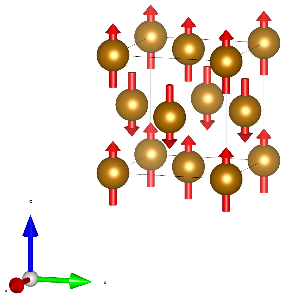
Fig. 12 Ball and stick model of iron (fcc) with antiferromagnetic.¶

Here we can define a unit cell with two Fe atoms, both having opposite spin magnetic moment.

Simulations¶

Hint

Enter the directory ‘02_Fe_fcc’

Prepare the input file for fcc iron. Initialize the spin magnetic moments of the Fe atoms to create antiferromagnetic order.
Run SIESTA The calculation should only take a few seconds (about 15 sec on 4 cores).

Hint

You can assign maximum spin polarization by using just the + and - symbols. So for this case, instead of:

%block DM.InitSpin
   1  4.0
   2 -4.0
%endblock DM.InitSpin

You can just write:

%block DM.InitSpin
   1  +
   2  -
%endblock DM.InitSpin

Analysis¶

What is the final spin magnetic moment in the unit cell? On each Fe atom?
Does the final magnetic phase match what you expected?
Compare the results for the antiferromagnetic structure to the ferromagnetic one. In which phase are the magnetic moments on the Fe atoms larger?

Note

The total energy of the calculation for fcc and bcc iron cannot be compared directly to determine which phase is lower in energy. The atomic structure in both calculation is fixed and comparing energies of the unrelaxed phases is not enough.

Spin-Orbit Coupling (10 min)¶

Goal of the exercise

Run a calculation with spin-orbit coupling (SOC), and analyze the results.

Note

When performing a calculation with spin-orbit coupling it is crucial to:

carefully converge the k–points sampling.
carefully converge the mesh cut-off.
converge the density matrix with a tolerance below 10^-5.
use relativistic pseudopotentials (PPs) and use the non–linear core corrections when the PPs are built.

All of the information regarding the basis set and all the parameters used in a common SIESTA calculation are also valid for the SOC.

In the examples here the above mentioned parameters (mesh cutoff, etc) are not converged because we want to speed up the calculations to show initial (and dirty) results, but remember, for a real calculation those values have to be converged.

An additional advice: remember to read the SOC section in the main SIESTA manual!

In this example, we will have a look at an isolated Fe atom. When the Dirac equation for an isolated iron is solved, the degeneracy of different states with the same $(n,l)$ quantum numbers should be lifted due to the coupling of the spin and orbital moments of the electrons. When we include relativistic effects, i.e. perform a calculation with spin-orbit coupling, we should be able to recover this splitting of the Fe($3d$) states.

Simulations¶

Hint

Enter the directory ‘03_Fe_isolated’

Run a calculation a fully relativistic calculation (setting Spin spin-orbit) and one scalar relativistic calculation (setting Spin polarized or Spin non-colinear) The calculations should only take a few seconds (about 10 sec on 4 cores).

Analysis¶

Compare the eigenvalues reported in the SIESTA output for the calculation scalar relativistic case (Spin polarized) and the fully relativistic case (Spin spin-orbit). In the scalar relativistic case there are 5 nearly degenerate eigenstates for both spin channels corresponding to the Fe($3d$). These states are not exactly degenerate due to the finite size of the simulation box, which gives rise to a small crystal field splitting. For the cubic shape of our simulation box the orbitals should be split into one group of 3 orbitals and one group of 2. In the fully relativistic case, this degeneracy should be fully lifted.

The eigenvalues will appear in the SIESTA output, because we specified WriteEigenvalues T in the input. For the scalar relativistic calculation they should look similar to this:
```
siesta: Eigenvalues (eV):
  ik is       eps
   1  1   -6.3406   -6.3406   -6.3406   -6.3366   -6.3366   -4.6726    0.3484    0.3484    0.3484   14.8135
          28.0972   28.0972   28.0977   28.0977   28.0977
   1  2   -3.8849   -2.7327   -2.7327   -2.7321   -2.7321   -2.7321    0.9691    0.9691    0.9691   15.3313
          29.5846   29.5846   29.5868   29.5868   29.5868
```
The eigenvalues of the fully relativistic calculation should look similar to this:
```
siesta: Eigenvalues (eV):
  ik =     1
     -6.3851   -6.3639   -6.3610   -6.3228   -6.2395   -4.6718   -3.8841   -2.7728   -2.7631   -2.7444
     -2.7050   -2.6570    0.3127    0.3361    0.3890    0.9411    0.9673    1.0090   14.8139   15.3319
     28.0754   28.0795   28.0863   28.1078   28.1443   29.5617   29.5686   29.5781   29.6035   29.6313
```
Splitting of Fe-$3d$ levels: $6.3851-6.2395 eV \approx 0.15 eV$.

Note

In SIESTA, fully-relativistic calculations are always performed in the ‘non-colinear` spin formalism, i.e. SIESTA works with two-component spinor wavefunctions. In general, these wavefunctions have both spin-up and spin-down components, which may vary in amplitude depending on the position in space. A distinction between spin-up and spin-down wavefunctions is, thus, generally not applicable. For this reason calculation with ‘non-colinear` spins, the eigenvalues are not separated by spin up (is=1) and spin down (is=2).

Magnetic anisotropy (15 min)¶

Goal of the exercise

Manipulate the direction of the initial spin moments.

In this example, you will calculate the magnetic anisotropy of a Pt₂ dimer. This means you will have to run multiple SIESTA calculations each with magnetic moments aligned along different directions and extract the total energy.

For this purpose, you will have to use the block DM.InitSpin. In non-colinear spin/spin-orbit calculation this block can be used to specify the initial direction of the spin moments in addition to their magnitude. The initial spin moment should be specified in spherical coordinates ($|S|, \theta, \phi$) (for more info on spherical coordinates see here).

%block DM.InitSpin
# atom index,  |S|, theta,  phi
           1   4.0    0.0   0.0
           2  -4.0   90.0  45.0
%endblock DM.InitSpin

Simulations¶

Hint

Enter the directory ‘04_Pt2’

To get started inspect the input file pt2_spin_z.fdf, and familiarize yourself with the options specified within.

Note

To speed the calculation, we are using reduced parameters which allow us maintain reasonable quality for the results. The original (converged) input options for this example can be found in pt2_spin_z.original.fdf. Can you see the differences?

Note

We sped up the calculations further by fine-tuning the mixer options. However, convergence is system is a bit tricky. So, it might still take a minute or two for each calculation to finish.

Use the input file and the pseudopotential of Pt atom, Pt.psf, and calculate the total self-consistent total energy E^tot for three highly symmetric orientations of the initial magnetization, (spin moment aligned along $x, y, z$). The two moments of the two atoms should always point in the same direction. Keep the atomic positions and the cell parameters fixed.

Hint

Remember to run each calculation in a separate folder, and do not do not re-use the density matrix (.DM file) obtained in other orientations. Reading the density matrix will cause SIESTA to ignore the DM.InitSpin. To calculate the total energy for different specific magnetic configuration you need to start from scratch.

After each calculation, check the final magnetic moments and ensure that they are pointing in the correct direction.

Change the orientation of the dimer (orient it along the $z$ or $y$ axes) and compute again the total energy again. This time keep the initial spin moments aligned along $z$.

Analysis¶

Compare the total energies for the different alignments of spin moment and the dimer axis. Some of the total energies should be the same, ignoring numerical fluctuation ( $< 1meV$). - In which cases are the total energies the same? - What do these cases have in common?
How large is magnetic anisotropy energy (the change in the total energy depending on the spin direction)?
What would happen if you used Spin non-colinear instead of Spin spin-orbit? Would you obtain the same values?

Hint

If you are not sure, you can try to change the Spin flag in the input and re-run SIESTA.

Advanced¶

What happens if you set initial configuration up in such a way that the spin moment and the dimer axis form an angle diffrent from 0 degress or 90 degrees (e.g. 20 degree)? Does the angle remain the same through-out the calculation?

Hint

The following exercises include additional analysis methods for SIESTA calculations with spin.

Visualizing the spin density (15 min)¶

In this example, you are going to perform calculations for a very small molecule: methyl CH₃. This molecule is a radical, i.e. it contains an unpaired electron. As a result, the molecule should exhibit spin polarization.

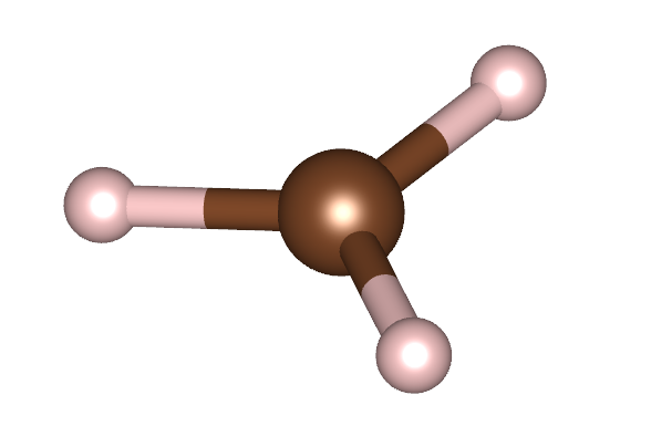
$(Ball and stick model of a methyl (CH\ :sub:`3`) molecule.)$

Fig. 13 Ball and stick model of a methyl (CH₃) molecule. White atoms: hydrogen; brown atom: carbon¶

Simulations¶

Hint

Enter the directory ‘05_CH3’

Perform calculations of the CH₃ molecule without spin and with collinear spins. Save the Mulliken charges and the charge density.

Analysis¶

How large is the spin magnetic moments of the molecule?
How does the total energy of the two calculations compare? What does the difference in total energy imply for the magnetic moment of ground state of the methyl radical?
Analyze on which Atoms and orbitals the spin magnetic moment is primarily localized.
Visualize the magnetic density (difference between spin-up charge density and spin-down density). We recommend using denchar (see here) or sisl (see here). Is the result consistent with the shape of the orbitals where the spin moment is localized?

Hint

We have provided an example input file (ch3.denchar.fdf) for denchar that you can use. denchar will produce multiple .CUBE files which can be visualized using various crystallgrahpic software. An explanation of each output file can be found in the denchar documentation.

The magnetic density (ch3.RHO.UPminusDOWN.cube) should look something like this

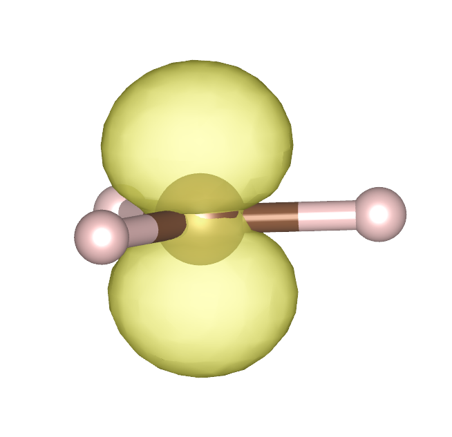
$(Spin density and ball-and-stick model of a methyl (CH\ :sub:`3`) radical.)$
Fig. 14 Spin density and ball-and-stick model of a methyl (CH₃) radical. White atoms: hydrogen; brown atom: carbon¶

Spin resolved density of states (30 min)¶

Goal of the exercise

Learn how to…

use the DM.InitSpin block to simulate the same material with different magnetic order.
extract the spin magnetic moment for each atom.
analyze the spin-resolved projected density of states.

Introduction¶

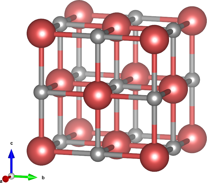
Fig. 15 Crystal structure of manganese oxide. Grey atoms: oxygen; red atoms: manganese¶

In this exercise we will work on a crystal structure consisting of magnetic (Mn) and non-magnetic atoms (O), specifically manganese oxide (MnO). Manganese oxide exhibites magnetism due to the partially filled 3d shells on the Mn atoms. MnO exhibits different (metastable) magnetic phases, which we can explore. By comparing the total energy of the different magnetic phases we can identify the “correct” magnetic phase.

We will consider three different magnetic phases:

FM has ferromagnetic order, that is all Mn atoms have the same spin orientation
AF1 has, what is called, the [001] ordering, that is, all Mn atoms in a given [001] plane are equivalent (has the same spin orientation), and between the consecutive [001] planes the spin orientations alternate.
AF2 has the [111] ordering, that is, equivalent spin orientation is throughout a given [111] plane and alternates between such planes.

Fig. 16 Crystal structure of manganese oxide with [001] (left) and [111] (right) antiferromagnetic order. Grey atoms: oxygen; red atoms: manganese (spin up); blue atoms: manganese (spin down).¶

Note

One complication with 3d oxides is that the real crystal structure, which very closely resembels the B1 (NaCl) type, undergoes slight but noticeable distortions which help to stabilize one or another magnetic phase. However, in the historical context as well as for didactic purposes, conventional DFT calculations, done in a nominally cubic lattice, play an important role.

Neglecting very small distortions that occur in different magnetic phases, MnO has a B1 (NaCl) structure. The latter is described in the input file as follows:

LatticeConstant     4.43 Ang
%block LatticeVectors
   0.00     0.50      0.50
   0.50     0.00      0.50
   0.50     0.50      0.00
%endblock LatticeVectors

AtomicCoordinatesFormat ScaledCartesian
%block AtomicCoordinatesAndAtomicSpecies
   0.000   0.000   0.000  1   # Mn
   0.500   0.500   0.500  2   # O
%endblock AtomicCoordinatesAndAtomicSpecies

The lattice constant is set at the experimental value, and kept constant throughout the present exercise.

In order to run a spin-polarized calculation, we set:

Spin                    polarized

and initialize non-zero (in fact, maximal) spin on Mn site:

%block DM.InitSpin       # Initial magnetic order (on Mn only)
   1   +
%endblock DM.InitSpin

Warning

When using the block DM.InitSpin, all atoms that are not listed explicitly inside the block will initially be non-magnetic. This behavior is opposite to the behavior when the DM.InitSpin block is not used at all. In the latter case, all atoms will initially have the largest possible spin magnetic moment.

The rest of the input file…

sets calculation parameters: GGA, k-mesh, mesh cutoff, …
enables additional outputs: Mulliken populations, charge (and magnetic) density, (projected) density of states

Charge.Mulliken end                # Output Mulliken charges after calculation finished
Charge.Mulliken.Format 1           # Output Mulliken per atoms and orbital
SaveRho                            # Save the charge density
%block ProjectedDensityOfStates    # Calculate the projected density of states
   -25.0  10.0  0.1   700   eV
%endblock ProjectedDensityOfStates

This part of the input file will be the same for the calculations with different magnetic orderings.

Simulations¶

Hint

Enter the directory ‘06_MnO’

Run a SIESTA calculation for MnO with ferromagnetic order.
Prepare the input files for the antiferromagnetic structures Note that an antiferromagnetic ordering doubles the unit cell: it contains now two Mn atoms (with opposite spins) and, correspondingly, two O atoms. Don’t forget to introduce changes in the lattice vectors and atomic coordinates.

Hint

Run calculations for each magnetic order in separate subfolders and save the SIESTA output there to review and compare them.

In case you struggle with this step, you can have a look at the input files in the Answers folder.
Run a SIESTA calculations for the antiferromagnetic structures.

Analysis¶

Check the local (on Mn and O sites) and total (per unit cell) magnetic moments for all three cases. On which atoms/atomic shells is the magnetic moment localized?
Compare the total energy of all three magnetic phases, which one is the most stable?
Check that the antiferromagnetic structures have pronounced band gaps.
Plot the spin-resolved density of states.
Hint

The gnuplot script plot_DOS.gplot can help with the visualization.
```
gnuplot -c plot_DOS.gplot MnO # Use gnuplot to plot the density of states
```
Note
- For Spin none the .DOS file contains two columns: energy and DOS.
- For Spin polarized the .DOS file contains three columns: energy, DOS↑, DOS↓ (DOS for spin-up/spin-down electrons). The integral of DOS↑ (DOS↓) up to E_F will give the number of electrons with spin-up (spin-down). The total density of states is the sum of DOS↑ and DOS↓.
- For Spin non-colinear or Spin spin-orbit the .DOS file contains five columns: energy, DOS↑, DOS↓, Re{DOS↑↓} and Im{DOS↑↓}.
The integral of Re{DOS↑↓} up to E_F will give the magnetization along X axis, Mx, and the integral of Im DOS↑↓ up to E_F , My. The total density of states is the sum of DOS↑ and DOS↓.
Plot the projected density of states for Mn and O separately.

Detailed information on calculating and visualizing the projected density of states can be found in this how-to and here.

Here, use the fmpdos utility, which provides an easy way to obtain the density of states for a given set of atoms/orbitals. For example, the density of states projected on the first manganese atom can be obtained like this:
```
$ fmpdos
  Input file name (PDOS):
MnO_FM.PDOS
  Output file name :
Mn1.PDOS
  Extract data for atom index (enter atom NUMBER, or 0 to select all),
  or for all atoms of given species (enter its chemical LABEL):
1
  Extract data for n= ... (0 for all n ):
0
```
The output file produced by fmpdos will have the same format as the .DOS file produced by siesta.
Hint

The gnuplot script plot_PDOS.gplot can help with the visualization.
```
gnuplot -c plot_PDOS.gplot MnO  # Use gnuplot to plot the density of states
```