Molecular dynamics

Do you want to get all tutorial materials on your local machine?

You can get all files and set up your local environment. Do that now before proceeding.

This tutorial provides an overview of the methods available in SIESTA for molecular dynamics, which includes the most common ensembles available in other codes that allow for molecular dynamics runs.

Take me to the exercises!

background Background Information

Additional information: Slides

These slides from previous presentations might help improve your understanding of the concepts presented in this tutorial:

• Presentation by Emilio Artacho

• Presentation by Marivi Fernadez-Serra

Molecular dynamics (MD) is a simulation method used to study the physical movements of atoms and molecules. It allows us to observe the behavior of molecules over time by solving Newton’s equations of motion for a system of interacting particles. Average quantities can then be extracted by doing postprocessing analysis over the generated trajectory. Instead of looking for minima at the potential energy surface (PES), MD aims to sample as many configurations as possible, moving over the PES. The image below shows the difference between a geometry optimization and a molecular dynamics run:

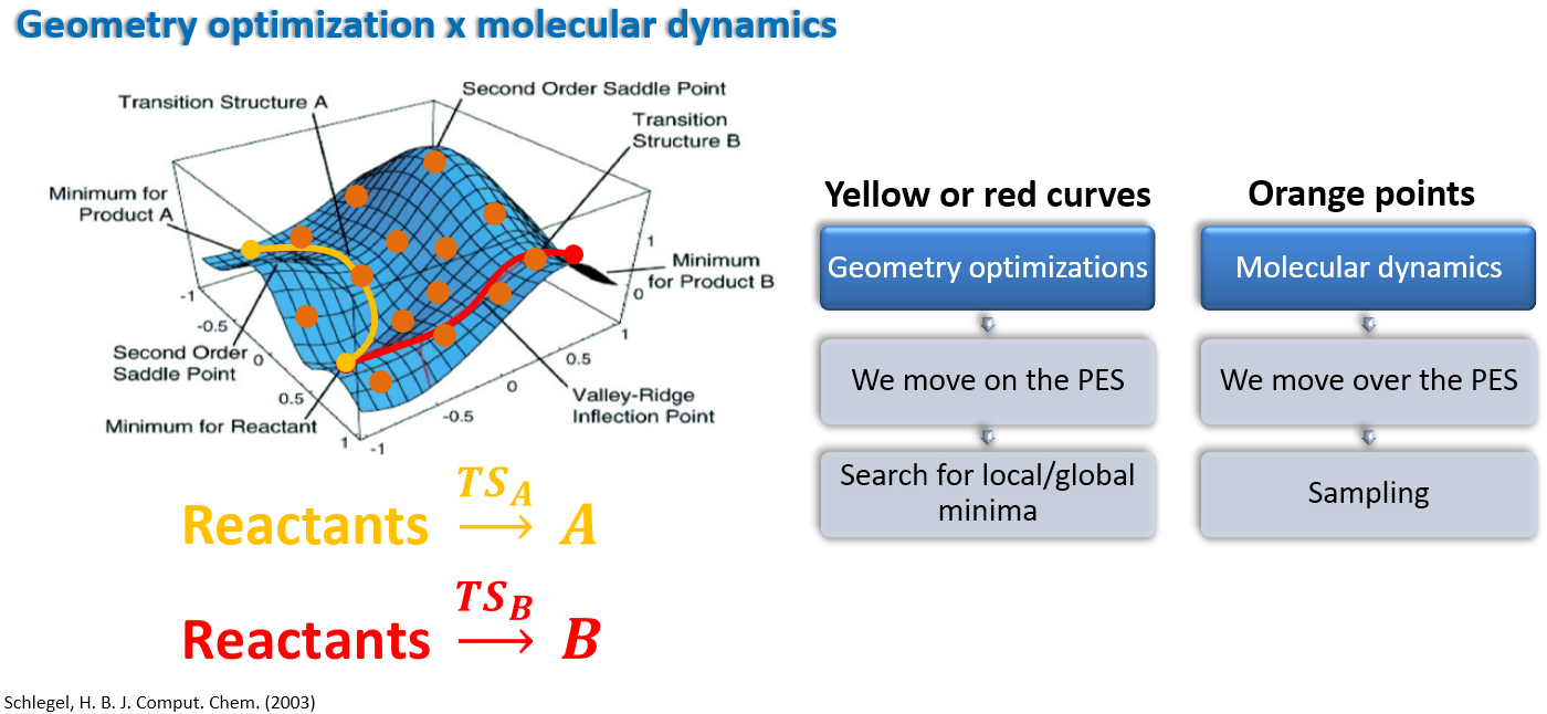
As one can see, the geometry optimization (GO) is a search for the minimum energy configuration of a system, while the molecular dynamics (MD) run is a simulation of the system over time. In the case of GO, the yellow and red curves in the image above exemplify two possible minimal energy reaction paths. The MD run, instead, is not limited to a single minimum, but rather explores the potential energy surface (PES) by moving through different configurations of the system, illustrated as the orange points in the image above.

When we run MD simulations, we can track the positions and velocities of atoms and molecules. The forces are computed for each new configuration, and this is the main aspect that is used to distinguish classical MD from ab initio MD. Those forces are then used to move the atoms. Therefore, SIESTA is capable of running ab initio MD simulations under different ensembles, which can be selected via the flag MD.TypeOfRun. With this very option, you choose what kind of dynamics you wish to run:

• Coordinate relaxations include are CG, Broyden, and FIRE (which are covered in Structural optimization using forces and stress).

• Options for regular molecular dynamics can be chosen through Verlet (NVE), Nose (NVT), ParrinelloRahman (NPE), and NoseParrinelloRahman (NPT). These are new options that will be explored in this tutorial.

Note

For molecular dynamics, the file *.ANI contains all of the structures generated during the relaxation in XYZ format. It can be processed by various graphical tools, such as Ovito, XCrysden or VMD.

The SystemLabel.ANI file do not include information about the simulation box. If you want to visualize the box, you can use the SystemLabel.MD file, which contains information about the cell vectors and their time derivatives. This file, however, is not in a standard format, so you will need to convert it to a format that your visualization program can read. For instance, you can use the md2axsf utility to convert the SystemLabel.MD file to an SystemLabel.AXSF file, which can be read by many visualization programs.

If you want to plot energy, pressure and temperature across the molecular dynamics run, you can use the scripts available in plotscripts under this same tutorial folder.

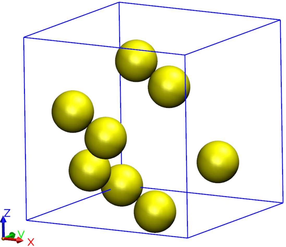
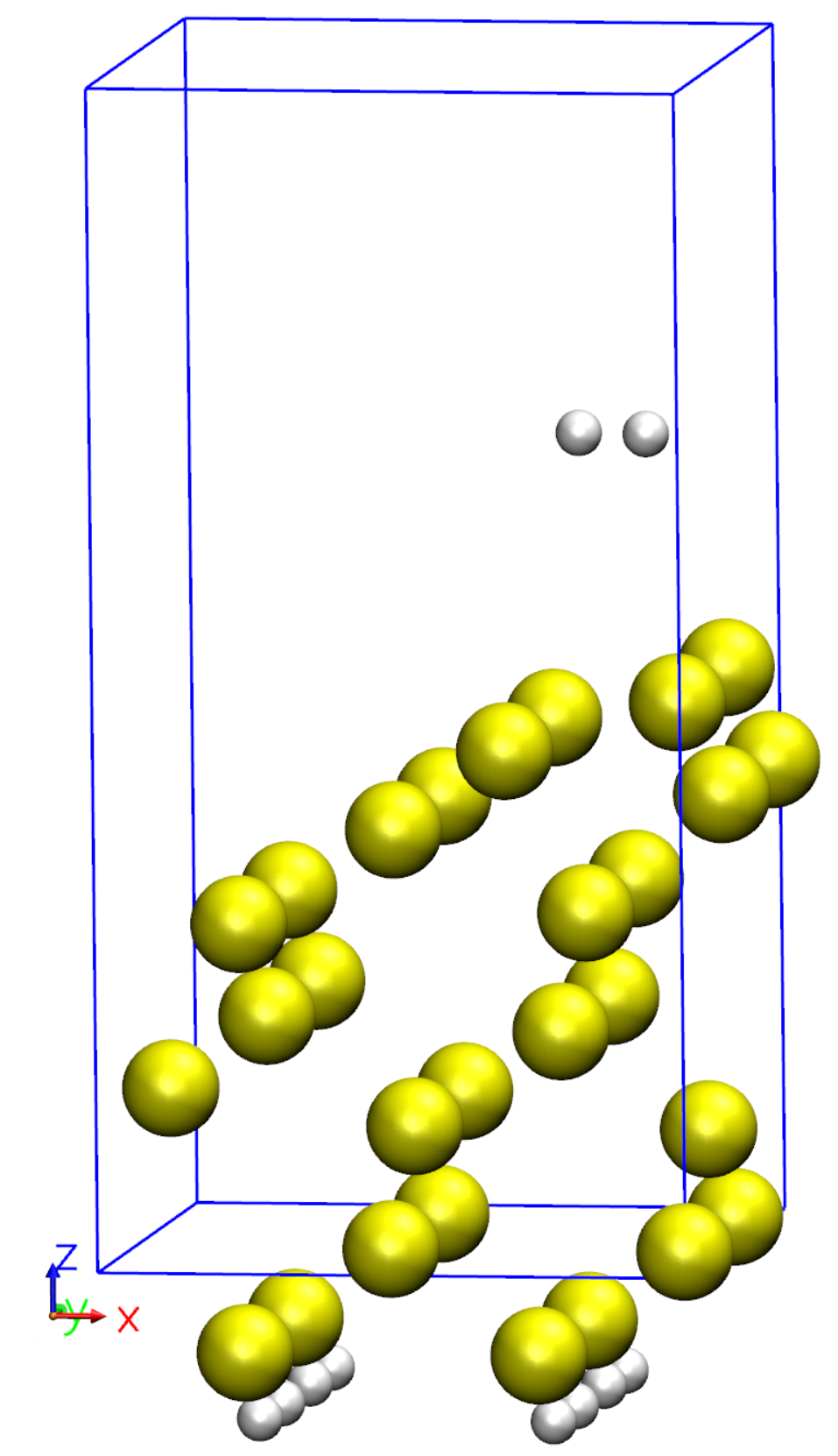
We will cover here four types of molecular dynamics: Verlet (NVE), Nose (NVT), Parrinello-Rahman (NPE), and Annealing. Examples for running molecular dynamics simulations are described below. The first three exercises utilize a Silicon supercell in the diamond structure. The Annealing example is done using a Silicon surface terminated with Hydrogen atoms. In the final example, we use quenched molecular dynamics for optimizing the geometry. For efficiency, the basis size is only a single-\(\zeta\) basis with short orbitals.

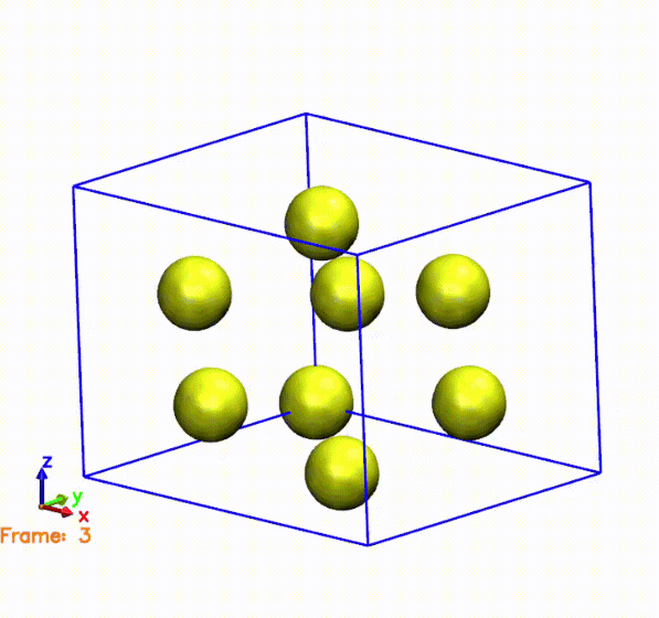
Silicon supercell used for the first three exercises and the quenched MD example:

Silicon surface with Hydrogen atoms used for the last example:

basic Verlet Dynamics (NVE)

Are you under a local environment?

Enter directory 01-Verlet

As usual, we have our fdf input file and our pseudopotentials:

• Pseudo: Si.psml

• Input file: si8.fdf

A peek at the fdf file

SystemName          Si - 8 atoms supercell
SystemLabel         si8

NumberOfAtoms       8
NumberOfSpecies     1

%block ChemicalSpeciesLabel
 1  14  Si
%endblock ChemicalSpeciesLabel

PAO.BasisSize       SZ
PAO.EnergyShift     300 meV

LatticeConstant     5.535 Ang

%block LatticeVectors
  1.000  0.000  0.000
  0.000  1.000  0.000
  0.000  0.000  1.000
%endblock LatticeVectors

MeshCutoff          30.0 Ry

%block kgrid_Monkhorst_Pack
   2  0  0  0.0 
   0  2  0  0.0 
   0  0  2  0.0 
%endblock kgrid_Monkhorst_Pack 

MaxSCFIterations    50  
DM.MixingWeight     0.3 
DM.NumberPulay      3  
DM.Tolerance        1.d-4
DM.UseSaveDM             

SolutionMethod         diagon    
ElectronicTemperature  25 meV  

MD.TypeOfRun           Verlet
MD.InitialTimeStep     1
MD.FinalTimeStep       200
MD.LengthTimeStep      3.0 fs
MD.InitialTemperature  300.0 K

WriteMDHistory T

AtomicCoordinatesFormat  ScaledbyLatticeVectors

%block AtomicCoordinatesAndAtomicSpecies
    0.000    0.000    0.000   1 #  Si  1
    0.250    0.250    0.250   1 #  Si  2
    0.000    0.500    0.500   1 #  Si  3
    0.250    0.750    0.750   1 #  Si  4
    0.500    0.000    0.500   1 #  Si  5 
    0.750    0.250    0.750   1 #  Si  6 
    0.500    0.500    0.000   1 #  Si  7 
    0.750    0.750    0.250   1 #  Si  8 
%endblock AtomicCoordinatesAndAtomicSpecies

For the purposes of running this example quickly, we are using a SZ basis set and a very low cutoff. You might want to move beyond this later, but there should not be qualitative changes in the results. Take a close look at the .fdf file within, in particular this section:

MD.TypeOfRun           Verlet
MD.InitialTimeStep     1
MD.FinalTimeStep       200
MD.LengthTimeStep      3.0 fs
MD.InitialTemperature  300.0 K

WriteMDHistory T

Note the MD options selected: the Verlet run will run for 200 steps with a timestep of 3.0 fs. The initial velocities are selected to correspond to a temperature of 300 K; in essence, this means that the atoms are assigned random velocities drawn from the Maxwell-Bolzmann distribution for that temperature. A constraint of zero center of mass velocity is imposed.

Also note the WriteMDHistory option, which is toggled to true. This means that SIESTA accumulates the molecular dynamics trajectory in the following files:

• SystemLabel.MD: atomic coordinates and velocities (and lattice vectors and their time derivatives, if the dynamics implies variable cell). The information is stored unformatted for postprocessing with utility programs to analyze the MD trajectory.

• SystemLabel.MDE: shorter description of the run, with energy, temperature, etc., per timestep.

These files are cumulative, so you can always restart the simulation for more sampling if the appropriate files are in a given directory. The files needed for a seamless restart are the SystemLabel.X_RESTART file (where X is some label corresponding to chosen dynamics option, such as VERLET or NOSE) and the SystemLabel.XV file, which stores current velocities and predicted positions for the next step. One can restart with just the SystemLabel.XV file as well, but it will be essentially re-setting the information related to thermostats, barostats and velocity propagators.

You can run the input file as usual:

$ siesta < si8.fdf > si8.out

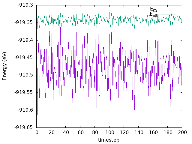
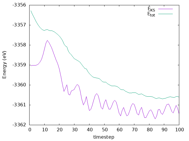
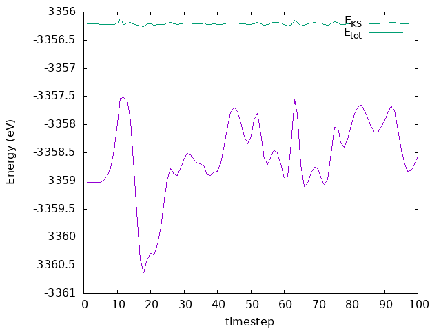
The run should not take very long. Now look at the resulting files in the directory: the SystemLabel.VERLET_RESTART and SystemLabel.XV files have been produced, so if you re-run SIESTA, it will add more configurations and information to the trajectory and SystemLabel.MDE files, respectively. Plot the total and Kohn-Sham energies from the si8.MDE file as a function of timestep. Is energy conserved? How large are the fluctuations? If you want to plot with gnuplot, you can use this plot script. You can use it by providing the output file as an argument:

$ ./plot_energies.sh

Answer: Is energy conserved? How large are the fluctuations?

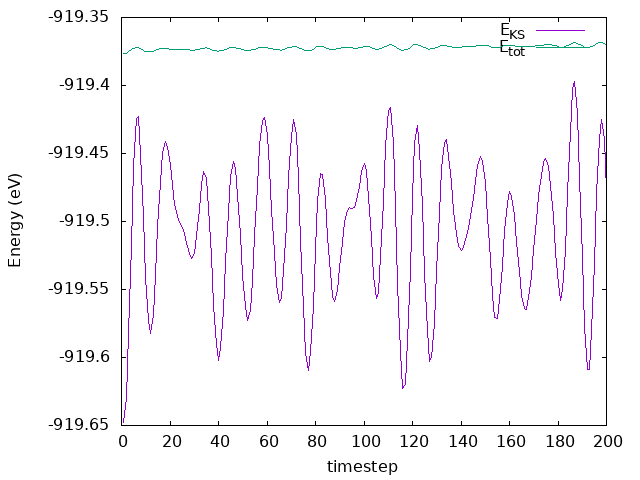
As we can see in the plot, the energy fluctuates around an average value, and the fluctuations are very small. Thereby, the energy is conserved.

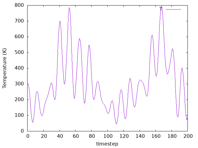
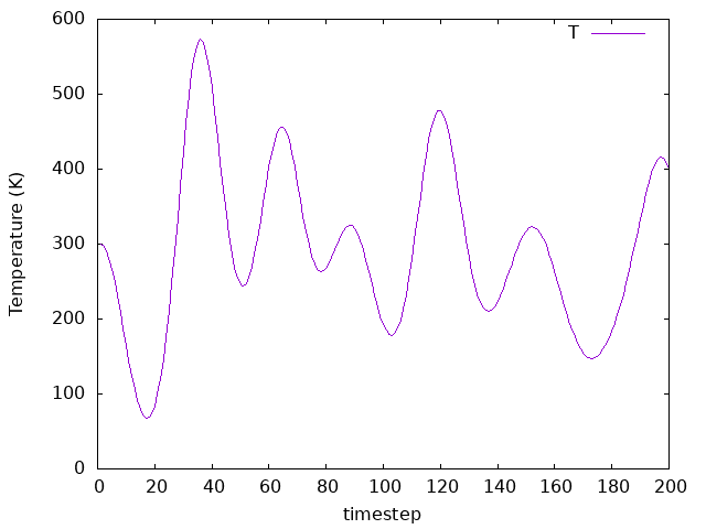
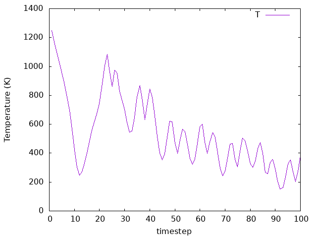
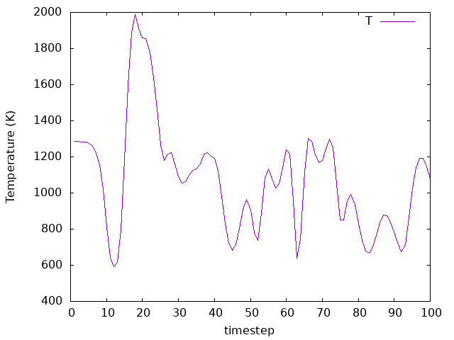
Now look at the temperature as a function of time. Look also at the pressure, to see what happens to it. How does temparature change as the system evolves? If you want to plot with gnuplot, you can use this plot script. You can use it by providing the output file as an argument:

$ ./plot_temp.sh

Answer: How does temparature change as the system evolves?

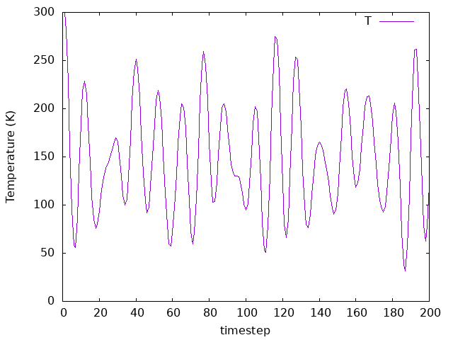
The temperature fluctuates as well, but since we don’t have a thermostat to control it, its value will not converge to an average number.

Now try re-running the system with a larger timestep (say, 10 fs). You need to change the MD.LengthTimeStep variable in the fdf file. Make sure to change the SystemLabel before re-running this time (or back up your previous results), so you can compare plots from separate files.

Answer: How does the system respond?

The fluctuations observed for both the energies and temperature are still there, but now we can see more “noise”. That’s because with 10.0 fs as a time step instead of 3.0 fs, we are reaching longer simulation times. In total, for 10 fs as a time step we are reaching 2 ps in total instead of 0.6 ps. Please note that increasing the time step for real simulations need further considerations. For example, to simulate water dynamics a time step of 1 fs is usually required.

Additional information: Visualizing your MD trajectory - highly recommended.

Enabling the WriteCoorXmol option (WriteCoorXmol T) will produce an XYZ-formatted file with the *.ANI extension.

For geometry optimizations, the file SystemLabel.ANI contains all the structures generated during the relaxation. For MD, it will contain the structures of each time step. This file format can be processed by various graphical tools, such as XCrysden , VMD or Ovito.

If you want to visuzlize the simulation box as well, you can use the SystemLabel.MD file, but it needs to be converted to a format that your visualization program can read. That can be done using the md2axsf utility to convert the SystemLabel.MD file to an AXSF file, for instance.

Below you can find a gif image generated using VMD. The same can be done using other codes at your convinience.

basic Nose Dynamics (NVT)

Are you under a local environment?

Enter directory 02a-Nose-300-100

As usual, we have our fdf input file and our pseudopotentials:

• Pseudo: Si.psml

• Input file: si8.fdf

A peek at the fdf file

SystemName          Si - 8 atoms supercell
SystemLabel         si8

NumberOfAtoms       8
NumberOfSpecies     1

%block ChemicalSpeciesLabel
 1  14  Si
%endblock ChemicalSpeciesLabel

PAO.BasisSize       SZ
PAO.EnergyShift     300 meV

LatticeConstant     5.535 Ang

%block LatticeVectors
  1.000  0.000  0.000
  0.000  1.000  0.000
  0.000  0.000  1.000
%endblock LatticeVectors

MeshCutoff          30.0 Ry

%block kgrid_Monkhorst_Pack
   2  0  0  0.0 
   0  2  0  0.0 
   0  0  2  0.0 
%endblock kgrid_Monkhorst_Pack 

MaxSCFIterations    50  
DM.MixingWeight     0.3 
DM.NumberPulay      3  
DM.Tolerance        1.d-4
DM.UseSaveDM             

SolutionMethod         diagon    
ElectronicTemperature  25 meV  

MD.TypeOfRun            Nose
MD.InitialTimeStep      1
MD.FinalTimeStep        200
MD.LengthTimeStep       3.0 fs
MD.InitialTemperature   300.0 K
MD.TargetTemperature    300.0 K
MD.NoseMass             100.0 Ry*fs**2

WriteMDHistory T

AtomicCoordinatesFormat  ScaledbyLatticeVectors

%block AtomicCoordinatesAndAtomicSpecies
    0.000    0.000    0.000   1 #  Si  1
    0.250    0.250    0.250   1 #  Si  2
    0.000    0.500    0.500   1 #  Si  3
    0.250    0.750    0.750   1 #  Si  4
    0.500    0.000    0.500   1 #  Si  5 
    0.750    0.250    0.750   1 #  Si  6 
    0.500    0.500    0.000   1 #  Si  7 
    0.750    0.750    0.250   1 #  Si  8 
%endblock AtomicCoordinatesAndAtomicSpecies

Now we move on to constant volume, constant temperature dynamics. We will use the Nose thermostat, which provides a thermal bath coupled to the system. The magnitude of this coupling is controlled by the MD.NoseMass variable, as you can find in the fdf:

MD.TypeOfRun            Nose
MD.InitialTimeStep      1
MD.FinalTimeStep        200
MD.LengthTimeStep       3.0 fs
MD.InitialTemperature   300.0 K
MD.TargetTemperature    300.0 K
MD.NoseMass             100.0 Ry*fs**2

See that we also have a new option here, MD.TargetTemperature, which, as the name implies, sets the desired (average) temperature for the system. In a real production run, MD.NoseMass should be carefully chosen by testing how the system responds to it. This reference can be helpful in determining a reasonable value for it:

\(Q = g * K * T * t^{2} / (2 \pi^{2})\)

Here, g is 3 times the number of atoms (i.e. the degrees of freedom for the system), T is the target temperature, K is the Boltzmann constant, and t is the timescale of the dominant modes for the system itself (usually 1-10 fs for lighter atoms, 10-100 fs por heavier atoms).

You can run the input file as usual:

$ siesta < si8.fdf > si8.out

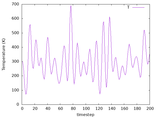
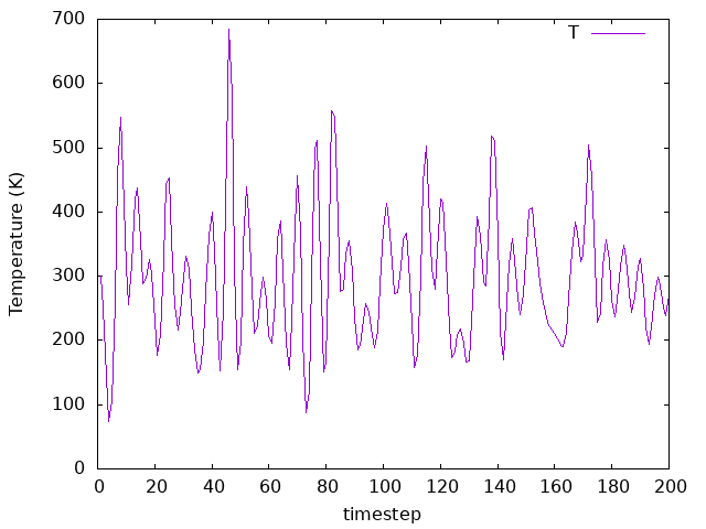
Run the system, and see how the temperature in the SystemLabel.MDE file behaves. If you want to plot with gnuplot, you can use this plot script. You can use it by providing the output file as an argument:

$ ./plot_temp.sh si8.out

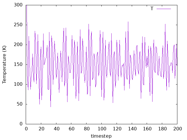
What’s happening to the temperature now as compared to the previous NVE example?

Answer: What’s happening to the temperature?

Now, the temperature fluctuates around the average of 300 K, which is the temperature we set. Please note that such high fluctuations are expected for a system of this size. You might want to increase the number of atoms in the system (e.g., replicate it 2x2x2 times) to see how the fluctuations decrease. However, that would demand a larger computational time, and that’s beyond the goal of this tutorial.

Now, create new directories, say 02b-Nose-300-10 and 02c-Nose-300-1. This is the same system as before, but change the MD.NoseMass to 10 Ry*fs**2 and 1 Ry*fs**2 respectively. You can download the modified fdf input files here (the pseudopotentials are the same as before):

• Pseudo: Si.psml

• Input file for MD.NoseMass 10 Ry*fs**2: si8.fdf

• Input file for MD.NoseMass 1 Ry*fs**2: si8.fdf

Are you under a local environment?

Enter directory 02b-Nose-300-10 and later to the directory 02c-Nose-300-1.

Run these examples as usual on their respective directories:

$ siesta < si8.fdf > si8.out

Once the simulations are completed, plot the temperature as a function of time-step to compare the effect the Nose mass has on a given target temperature. How does the average fluctuate across Nose masses? Try to plot the running average of the temperature over a given number of timesteps (i.e. 25). If you want to plot with gnuplot, you can use this plot script. You can use it by providing the output file as an argument:

$ ./plot_temp.sh si8.out

Answer: How does the average fluctuate across Nose masses?

MD.NoseMass 100 Ry*fs**2

MD.NoseMass 10 Ry*fs**2

MD.NoseMass 1 Ry*fs**2

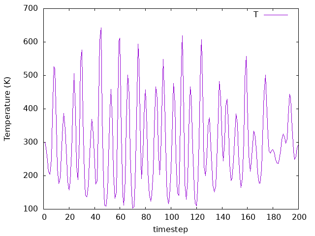
As you can see by comparing the three plots MD.NoseMass 100 Ry*fs**2, 10 Ry*fs**2, and 1 Ry*fs**2), the coupling affects how the temperature bath fluctuates. It’s value must be chosen according to the system you are investigating in a real simulation.

Finally, let’s change the target temperature for MD.NoseMass 10 Ry*fs**2. You can create a new directory, say 02d-Nose-600-10, and repeat the same procedure. You can download the modified fdf input file here (the pseudopotential is the same as before):

• Pseudo: Si.psml

• Input file: si8.fdf

Are you under a local environment?

Enter directory 02d-Nose-600-10.

Run this example as usual on its respective directory:

$ siesta < si8.fdf > si8.out

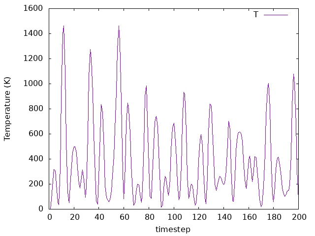
What changed as compared to the previous cases for MD.TargetTemperature 300.00 K ? See how the temperature in the SystemLabel.MDE file behaves. If you want to plot with gnuplot, you can use this plot script. You can use it by providing the output file as an argument:

$ ./plot_temp.sh si8.out

Answer: What changed as compared to the previous cases?

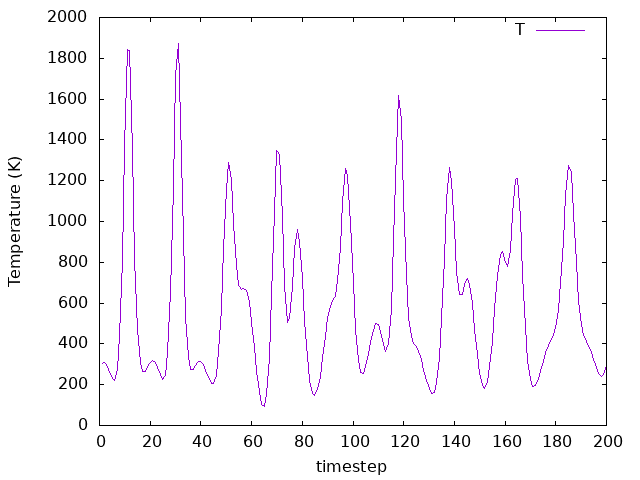
As it can be seen in the plot, now the MD.TargetTemperature is 600.00 K, but the MD.NoseMass is 10 Ry*fs**2. Therefore, a good value for the MD.NoseMass should be considered, and the equation presented before provides a good guess. Yet, now the temperature fluctuates around the new target temperature, which is what we want.

Now pick a simulation with a certain Nose mass to increase the timestep itself. (making sure to change the SystemLabel). Compare the results for different timesteps with the same Nose mass. How do the temperature values and the averages differ?

Answer: How do the temperature values and the averages differ?

MD.LengthTimeStep 1 fs

MD.LengthTimeStep 3 fs

MD.LengthTimeStep 5 fs

To perform this exercise, we chose the example on directory 02b-Nose-300-10, but you could choose any other example. We tested 2 different time steps, one smaller than the original and one bigger. Therefore, we can compare what happens to the temperature as we change the time step, as we can see in the above plots. As we can observe, the averages are similar for all time steps, but the fluctiations change significantly.

basic Parrinello-Rahman Dynamics (NPE)

Are you under a local environment?

Enter directory 03-ParrinelloRahman

As usual, we have our fdf input file and our pseudopotentials:

• Pseudo: Si.psml

• Input file: si8.fdf

A peek at the fdf file

SystemName          Si - 8 atoms supercell
SystemLabel         si8

NumberOfAtoms       8
NumberOfSpecies     1

%block ChemicalSpeciesLabel
 1  14  Si
%endblock ChemicalSpeciesLabel

PAO.BasisSize       SZ
PAO.EnergyShift     300 meV

LatticeConstant     5.535 Ang

%block LatticeVectors
  1.150  0.200  0.000
  0.000  1.050  0.000
 -0.100  0.000  0.900
%endblock LatticeVectors

MeshCutoff          30.0 Ry

%block kgrid_Monkhorst_Pack
   2  0  0  0.0 
   0  2  0  0.0 
   0  0  2  0.0 
%endblock kgrid_Monkhorst_Pack 

MaxSCFIterations     50  
DM.MixingWeight      0.3 
DM.NumberPulay       3  
DM.Tolerance         1.d-3
DM.UseSaveDM             

SolutionMethod         diagon    
ElectronicTemperature  25 meV  

MD.TypeOfRun            ParrinelloRahman
MD.InitialTimeStep      1
MD.FinalTimeStep        200
MD.LengthTimeStep       3.0 fs
MD.ParrinelloRahmanMass 10.0 Ry*fs**2
MD.TargetPressure       0.0 GPa

WriteMDHistory T

AtomicCoordinatesFormat  ScaledbyLatticeVectors

%block AtomicCoordinatesAndAtomicSpecies
    0.000    0.000    0.000   1 #  Si  1
    0.250    0.250    0.250   1 #  Si  2
    0.000    0.500    0.500   1 #  Si  3
    0.250    0.750    0.750   1 #  Si  4
    0.500    0.000    0.500   1 #  Si  5 
    0.750    0.250    0.750   1 #  Si  6 
    0.500    0.500    0.000   1 #  Si  7 
    0.750    0.750    0.250   1 #  Si  8 
%endblock AtomicCoordinatesAndAtomicSpecies

Now, instead of maintaining the constant temperature, we will keep constant pressure. This means that the cell sizes will change during the MD. Examine the above .fdf file. Now the MD.TypeOfRun is ParrinelloRahman, with corresponding options MD.ParrinelloRahmanMass and MD.TargetPressure:

MD.TypeOfRun            ParrinelloRahman
MD.InitialTimeStep      1
MD.FinalTimeStep        200
MD.LengthTimeStep       3.0 fs
MD.ParrinelloRahmanMass 10.0 Ry*fs**2
MD.TargetPressure       0.0 GPa

Here the MD.ParrinelloRahmanMass plays a similar role to the mass of the Nose thermostat. The settings set the desired system pressure to 0. Run this example as usual:

$ siesta < si8.fdf > si8.out

Now, examine the resulting pressures and temperatures. If you want to plot with gnuplot, you can use this plot script for pressure and this plot script for temperature. You can use them by providing the output file as an argument:

$ ./plot_energies.sh si8.out

$ ./plot_pressure.sh si8.out

Is zero pressure achieved? Check a running window average (with, say, 25 timesteps). How does the average look? What about the temperature? Check it and its average as well.

Answer: Is zero pressure achieved? What about the temperature? How does the average look?

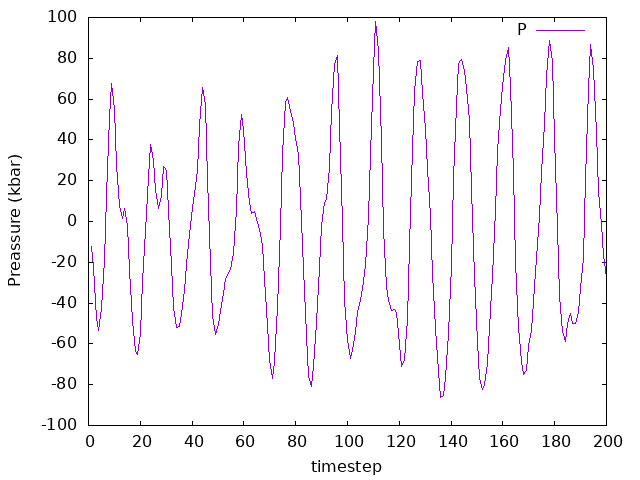
As we can see, on average the pressure is zero. Having a negative instant pressure might be a bit confusing here. What this really means in MD is that we are taking into account the direction in which the force is exerted (i.e., towards inside or outside the simulation box). As for the temperature, since there is no thermostat here (NPE ensemble), the system is not equilibrated to a given temperature.

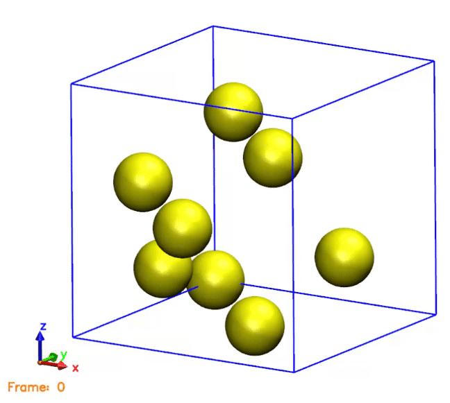
Now we want to see the behavior of the cell, but for that we will need to change our files to a format readable by other visualization programs. To examine the behavior of the unit cell, have it analyze the SystemLabel.MD file and output all the steps. Visualize the behavior of the atoms and the cell by running your favorite visualization program on the resulting trajectory file. Look at the steps where the cell seems particularly compressed, and compare it with the plot of pressure over time. Do the values make sense? What about steps where the cell is particularly expanded?

Answer: Do the values make sense? What about steps where the cell is particularly expanded?

The above gif was generated by postprocessing the SystemLabel.MD file with the md2axsf utility. After running the md2axsf tool, the system label was introduced, then the MD format was chosen, all the steps were selected by typing 0 0 0 and, finally, no output cell was defined, i.e., the cell dimensions were taken from the SystemLabel.MD file.

The gif shows the cell and atoms moving over time. If we compare the frames in the gif with the pressure plot, we can see that when the cell is compressed (i.e., the cell is smaller than the original one), the pressure is negative. This means that the system is being compressed, and the atoms are moving towards the center of the cell. On the other hand, when the cell is expanded (i.e., the cell is larger than the original one), the pressure is positive. This means that the system is being expanded, and the atoms are moving away from the center of the cell. This is consistent with the behavior of the pressure, which is negative when the cell is compressed and positive when the cell is expanded.

intermediate Annealing - Si(001) + H2 and Constraints

Are you under a local environment?

Enter directory 04-AnnealSiH2

As usual, we have our fdf input file and our pseudopotentials:

• Pseudos: Si.psml, H.psml

• Input file: Si001+H2.fdf

A peek at the fdf file

SystemName      Si001+H2
SystemLabel     Si001+H2

NumberOfSpecies        2
NumberOfAtoms          38

%block ChemicalSpeciesLabel
  1   1  H 
  2  14  Si 
%endblock ChemicalSpeciesLabel

%block AtomicMass
 1  2.013
%endblock AtomicMass

MeshCutoff    50.0 Ry         # Mesh cutoff. real space mes
XC.functional GGA
XC.Authors    PBE

Spin non-polarized

SolutionMethod    diagon    # OrderN or Diagon

MaxSCFIterations  300       # Maximum number of SCF iter
DM.MixingWeight   0.25      # New DM amount for next SCF cycle
DM.Tolerance      1.d-4     # Tolerance in maximum difference between input and output DM
DM.UseSaveDM      true      # to use continuation files
DM.MixSCF1        true
DM.NumberPulay    4

MD.TypeOfRun          Anneal
MD.InitialTimeStep    1
MD.FinalTimeStep      100
MD.LengthTimeStep     2.0 fs
MD.AnnealOption       Temperature
MD.TargetTemperature  300.0 K
MD.TauRelax           50.0 fs

MD.UseSaveXV   .true.
WriteMDhistory    .true.

%block GeometryConstraints
        position  from   19  to  38
%endblock GeometryConstraints

LatticeConstant  1.91587 Ang

%block LatticeVectors
 4.0     0.0     0.0
 0.0     4.0     0.0 
 0.0     0.0     8.0
%endblock LatticeVectors

AtomicCoordinatesFormat    Bohr

%block AtomicCoordinatesAndAtomicSpecies
      11.449096152       3.620202345      -8.313070747        1  H 
      13.106542549       3.621016654      -8.325506604        1  H 
       9.548438948       3.618923362     -16.541210979        2  Si
      13.817205862       3.620847822     -15.309180773        2  Si
       9.528270466      10.866602791     -16.580589107        2  Si
      13.790382977      10.846154693     -15.308839631        2  Si
       7.406101538      -0.000108928     -18.056395328        2  Si
      14.268039181      -0.000697920     -17.990731589        2  Si
       7.400674278       7.240493241     -18.092233975        2  Si
      14.268278001       7.238006697     -17.983063045        2  Si
       3.571414424      -0.000007639     -20.399498936        2  Si
      10.883283639      -0.000633692     -20.931428915        2  Si
       3.573258284       7.243442738     -20.425789208        2  Si
      10.889439123       7.235737400     -20.912814093        2  Si
       3.622183349       3.623006627     -23.077357499        2  Si
      10.864199345       3.618406638     -23.384919566        2  Si
       3.620283904      10.861372263     -23.080457914        2  Si
      10.865877628      10.862592010     -23.385099171        2  Si
       7.238876595       3.619448691     -25.736778053        2  Si
      14.477753190       3.619448691     -25.736778053        2  Si
       7.238012990      10.856486582     -25.737501819        2  Si
      14.482369793      10.860400206     -25.737284500        2  Si
       7.238876595       0.000000000     -28.310480236        2  Si
      14.477753190       0.000000000     -28.310480236        2  Si
       7.236705299       7.237017104     -28.310807159        2  Si
      14.474107907       7.237017104     -28.310778813        2  Si
       3.619448691       0.000000000     -30.884157853        2  Si
      10.858325286       0.000000000     -30.884157853        2  Si
       3.619424125       7.237026553     -30.883126062        2  Si
      10.866139307       7.237026553     -30.883137400        2  Si
       3.619535619       2.027521982     -32.725963147        1  H 
       3.619537508      -2.027482298     -32.725980154        1  H 
      10.858183557       2.026529876     -32.729474259        1  H 
      10.858183557      -2.026503419     -32.729461031        1  H 
       3.619509162       9.284967034     -32.733493708        1  H 
       3.621468809       5.196956784     -32.733510716        1  H 
      10.866137417       9.275867999     -32.720738052        1  H 
      10.862221903       5.200167430     -32.736386880        1  H 
%endblock AtomicCoordinatesAndAtomicSpecies

PAO.BasisType    split
PAO.BasisSize    SZ
PAO.EnergyShift  0.25 eV

PAO.NewSplitCode
PAO.FixSplitTable

We will cover now one last option for MD, which works specially well for system equilibration to a desired temperature and/or pressure. Look at the .fdf file in this final example. The system is now composed of Si atoms and H atoms, and the H atoms have been given the mass of deuterium to allow for a faster timestep. Besides annelaing the temperature, this example also cover another two aspects which might be very useful: the use of constraints and reading previous XV file. Note the MD options specified:

MD.TypeOfRun          Anneal
MD.InitialTimeStep    1
MD.FinalTimeStep      100
MD.LengthTimeStep     2.0 fs
MD.AnnealOption       Temperature
MD.TargetTemperature  300.0 K
MD.TauRelax           50.0 fs

This time, the dynamics will be simulated by annealing to the desired temperature, according to the specified relaxation time MD.TauRelax. Also, note the MD.AnnealOption variable; it can take the values of Temperature, Pressure and TemperatureAndPressure. The annealing method slowly takes the system from the initial to the desired conditions, using TauRelax as the characteristic time for the process. Beware that annealing is only recommended to equilibrate a system before moving on to other methods; taking MD-related properties (such as radial distribution functions) is not recommended since annealing will yield unphysical results. Independently from this, you will also find the following option in the fdf file:

MD.UseSaveXV   .true.

This means that SIESTA will attempt to find an SystemLabel.XV file to use as a restart, taking the initial coordinates and velocities from it. This will superceed the coordinates present in the fdf file and skip the initial random velocity generation (this means that MD.InitialTemperature will not have any effect if an .XV is found).

Hint

You can find a restart file called Si001+H2.XV under restart_files directory, or you can download it here. Copy it to your working directory every time you run a new simulation, so that you are always guaranteed to start from the same conditions.

Now, take a look at the Si001+H2.XV file. Which atoms are moving, and where are they moving towards?

Answer: Which atoms are moving, and where are they moving towards?

         14.481884133       0.000000000       0.000000000          0.000000000       0.000000000       0.000000000
          0.000000000      14.481884133       0.000000000          0.000000000       0.000000000       0.000000000
          0.000000000       0.000000000      28.963768267          0.000000000       0.000000000       0.000000000
          38
  1     1      11.449096152       3.620202345      -8.313070747          0.000000000       0.000000000      -0.220000000
  1     1      13.106542549       3.621016654      -8.325506604          0.000000000       0.000000000      -0.220000000
  2    14       9.548438948       3.618923362     -16.541210979          0.000000000       0.000000000       0.000000000
  2    14      13.817205862       3.620847822     -15.309180773          0.000000000       0.000000000       0.000000000
  2    14       9.528270466      10.866602791     -16.580589107          0.000000000       0.000000000       0.000000000
  2    14      13.790382977      10.846154693     -15.308839631          0.000000000       0.000000000       0.000000000
  2    14       7.406101538      -0.000108928     -18.056395328          0.000000000       0.000000000       0.000000000
  2    14      14.268039181      -0.000697920     -17.990731589          0.000000000       0.000000000       0.000000000
  2    14       7.400674278       7.240493241     -18.092233975          0.000000000       0.000000000       0.000000000
  2    14      14.268278001       7.238006697     -17.983063045          0.000000000       0.000000000       0.000000000
  2    14       3.571414424      -0.000007639     -20.399498936          0.000000000       0.000000000       0.000000000
  2    14      10.883283639      -0.000633692     -20.931428915          0.000000000       0.000000000       0.000000000
  2    14       3.573258284       7.243442738     -20.425789208          0.000000000       0.000000000       0.000000000
  2    14      10.889439123       7.235737400     -20.912814093          0.000000000       0.000000000       0.000000000
  2    14       3.622183349       3.623006627     -23.077357499          0.000000000       0.000000000       0.000000000
  2    14      10.864199345       3.618406638     -23.384919566          0.001005880       0.000000000       0.000000000
  2    14       3.620283904      10.861372263     -23.080457914          0.000000000       0.000000000       0.000000000
  2    14      10.865877628      10.862592010     -23.385099171          0.000000000       0.000000000       0.000000000
  2    14       7.238876595       3.619448691     -25.736778053          0.000000000       0.000000000       0.000000000
  2    14      14.477753190       3.619448691     -25.736778053          0.000000000       0.000000000       0.000000000
  2    14       7.238012990      10.856486582     -25.737501819          0.000000000       0.000000000       0.000000000
  2    14      14.482369793      10.860400206     -25.737284500          0.000000000       0.000000000       0.000000000
  2    14       7.238876595       0.000000000     -28.310480236          0.000000000       0.000000000       0.000000000
  2    14      14.477753190       0.000000000     -28.310480236          0.000000000       0.000000000       0.000000000
  2    14       7.236705299       7.237017104     -28.310807159          0.000000000       0.000000000       0.000000000
  2    14      14.474107907       7.237017104     -28.310778813          0.000000000       0.000000000       0.000000000
  2    14       3.619448691       0.000000000     -30.884157853          0.000000000       0.000000000       0.000000000
  2    14      10.858325286       0.000000000     -30.884157853          0.000000000       0.000000000       0.000000000
  2    14       3.619424125       7.237026553     -30.883126062          0.000000000       0.000000000       0.000000000
  2    14      10.866139307       7.237026553     -30.883137400          0.000000000       0.000000000       0.000000000
  1     1       3.619535619       2.027521982     -32.725963147          0.000000000       0.000000000       0.000000000
  1     1       3.619537508      -2.027482298     -32.725980154          0.000000000       0.000000000       0.000000000
  1     1      10.858183557       2.026529876     -32.729474259          0.000000000       0.000000000       0.000000000
  1     1      10.858183557      -2.026503419     -32.729461031          0.000000000       0.000000000       0.000000000
  1     1       3.619509162       9.284967034     -32.733493708          0.000000000       0.000000000       0.000000000
  1     1       3.621468809       5.196956784     -32.733510716          0.000000000       0.000000000       0.000000000
  1     1      10.866137417       9.275867999     -32.720738052          0.000000000       0.000000000       0.000000000
  1     1      10.862221903       5.200167430     -32.736386880          0.000000000       0.000000000       0.000000000

In the Si001+H2.XV file, we have both the coordinates and velocities. At the head of the file, the cell vectors and its velocities (if the cell changes) are printed. After that, each atom coordinate (columns 2, 3, and 4) and velocity (colums 5, 6, and 7) are printed. If you observe, all the velocities are zero apart from the first two, which corresponds to the Hydrogen molecule. Also, its velocity is negative and only along z direction. Therefore, one should expect the Hydrogen molecule to move towards the Si surface. However, if you do not copy the Si001+H2.XV file from the restart_files folder into the running directory, the initial velocities will be randomily generated for all atoms moving.

There is one last new thing in this fdf:

%block GeometryConstraints
        position  from   19  to  38
%endblock GeometryConstraints

This basically fixes the coordinates of the bottom half of the Si structure, so that only the surface interacting with Hydrogen molecule is allowed to move, accelerating the calculations. This block is very flexible and other variants can be found in the manual.

Run the example as usual:

$ siesta < Si001+H2.fdf > Si001+H2.out

It should take a bit longer to finish as compared to the previous exmaples. Now, visualize the trajectory file generated. Try to relate the trajectory with the Si001+H2.XV file you used. Does it make sense?

Answer: Does the trajectory make sense?

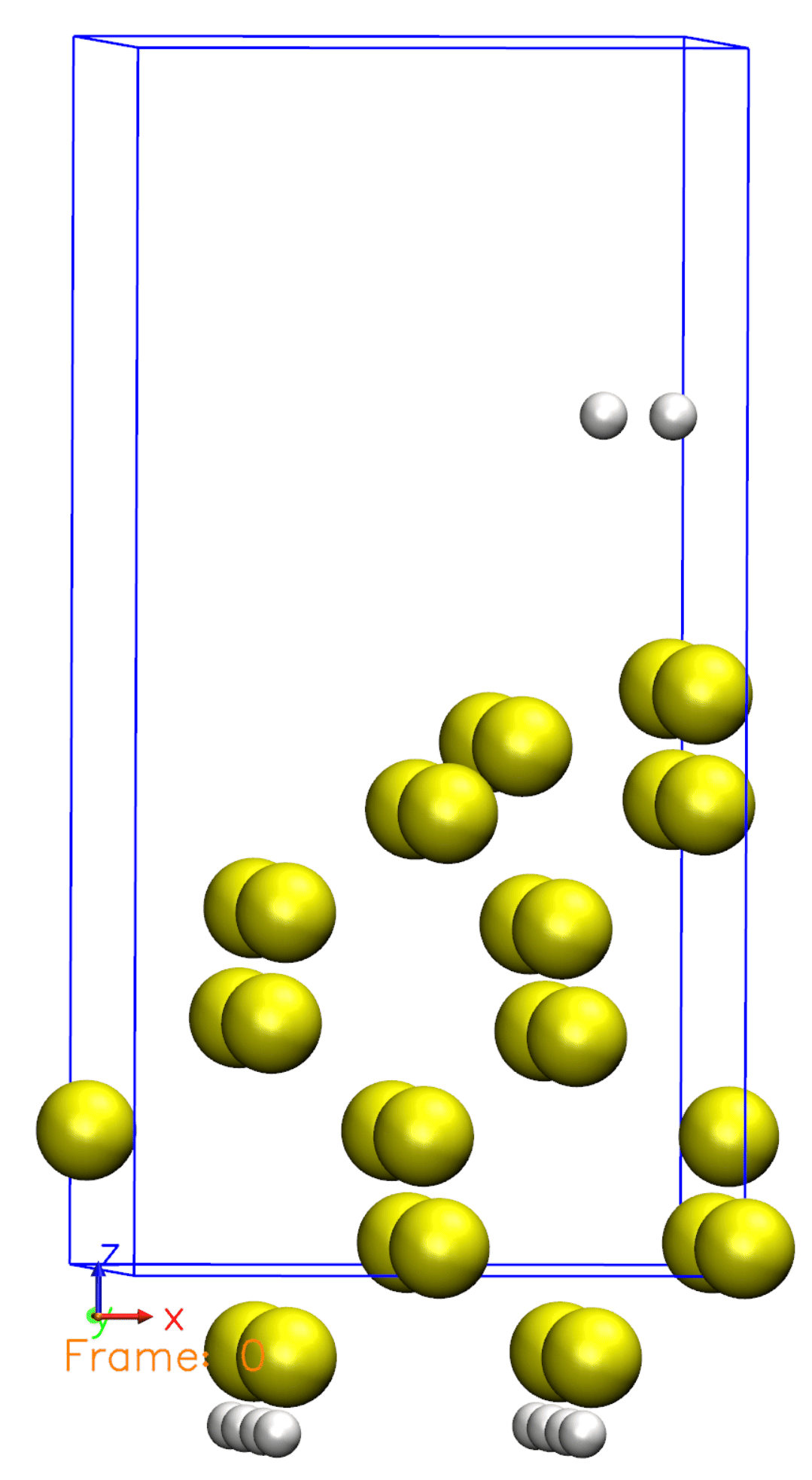
Just like we defined in the Si001+H2.XV file, the Hydrogen molecule is initially far from the surface and then starts to move towards the surface. Once reaching the surface, the molecule is then dissociated. You can also observe that some atoms are moving, but not all of them. This is because we defined a constraint for the bottom half of the atoms, so they are not allowed to move.

Now, take a look at the SystemLabel.MDE file. Is the desired temperature reached? How does the energy behave as the simulation progresses? If you want to plot with gnuplot, you can use this plot script for energy and this plot script for temperature. You can use them by providing the output file as an argument:

$ ./plot_ene.sh si8.out

$ ./plot_tempe.sh si8.out

Answer: Is the desired temperature reached? How does the energy behaves?

The temperature goes to the defined value as desired. If we run the simulation for longer, we would see it equilibrating where fluctuations around the defined valued would occur. As for the energy, it is not conserved, but it is decreasing. This is because the system is losing energy as the Hydrogen molecule is dissociating and the atoms are moving towards the surface. The energy is not conserved because we are using a thermostat to control the temperature, and the system is not in equilibrium. The energy is decreasing because the system is losing energy to the thermostat, which is trying to keep the temperature constant.

Now change the .fdf file to do simulate the NVE ensemble, using the Verlet algorithm as before (suggestion: change the name of SystemLabel to keep runs separate or create a new directory). Copy the Si001+H2.XV restart file and rename it to the appropriate filename; then, redo the simulation. Take another look at the SystemLabel.MDE file: How does it change? Is the energy conserved this time?

Answer: Is the energy conserved this time?

The temperature is not controlled anymore, and it fluctuates around a value that is not the same as the one we set. The energy is conserved, but it is not constant. The energy is not constant because the system is not in equilibrium, and the atoms are moving towards the surface.

intermediate Relaxation with Quenched Molecular Dynamics

Are you under a local environment?

Enter directory 05-quenched_md

As usual, we have our fdf input file and our pseudopotentials:

• Pseudo: Si.psml

• Input file: Si8.fdf

A peek at the fdf file

SystemName          Si - 8 atoms supercell
SystemLabel         si8

NumberOfAtoms       8
NumberOfSpecies     1

%block ChemicalSpeciesLabel
 1  14  Si
%endblock ChemicalSpeciesLabel

PAO.BasisSize       SZ
PAO.EnergyShift     300 meV

LatticeConstant     5.535 Ang

%block LatticeVectors
  1.150  0.200  0.000
  0.000  1.050  0.000
 -0.100  0.000  0.900
%endblock LatticeVectors

MeshCutoff          30.0 Ry

%block kgrid_Monkhorst_Pack
   2  0  0  0.0
   0  2  0  0.0
   0  0  2  0.0
%endblock kgrid_Monkhorst_Pack

MaxSCFIterations     50
DM.MixingWeight      0.3
DM.NumberPulay       3
DM.Tolerance         1.d-3
DM.UseSaveDM

SolutionMethod         diagon
ElectronicTemperature  25 meV

MD.TypeOfRun             ParrinelloRahman
MD.InitialTimeStep       1
MD.FinalTimeStep         200
MD.LengthTimeStep        3.0 fs
MD.ParrinelloRahmanMass  10.0 Ry*fs**2
MD.TargetPressure        0.0 GPa
MD.Quench                T

WriteMDHistory T

AtomicCoordinatesFormat  ScaledbyLatticeVectors

%block AtomicCoordinatesAndAtomicSpecies
    0.000    0.000    0.000   1 #  Si  1
    0.250    0.250    0.250   1 #  Si  2
    0.000    0.500    0.500   1 #  Si  3
    0.250    0.750    0.750   1 #  Si  4
    0.500    0.000    0.500   1 #  Si  5
    0.750    0.250    0.750   1 #  Si  6
    0.500    0.500    0.000   1 #  Si  7
    0.750    0.750    0.250   1 #  Si  8
%endblock AtomicCoordinatesAndAtomicSpecies

There is an alternative relaxation method that uses a physically motivated scheme, rather than a purely mathematical search for a ‘zero forces and stress’ configuration. Imagine that we perform a molecular dynamics simulation in which, rather than relaxing, we move the atoms, and the cell vectors, according to the (classical) equations of motion, using the forces and stress (see this tutorial). The trick in this case is that, every time an atom senses a force ‘opposite’ its velocity (in the sense that their scalar product is negative), the velocity is set to zero. This roughly corresponds to the idea: “since the atom seems to be moving away from its equilibrium point, we rather stop it”. The same can be done with strains and stress in the case of variable cell. Take a look now at the “relaxation section” of the si8.fdf file:

MD.TypeOfRun             ParrinelloRahman
MD.InitialTimeStep       1
MD.FinalTimeStep         200
MD.LengthTimeStep        3.0 fs
MD.ParrinelloRahmanMass  10.0 Ry*fs**2
MD.TargetPressure        0.0 GPa
MD.Quench                T

The ParrinelloRahman scheme is a combined atoms+cell microcanonical scheme (refer to the MD tutorial). We allow it to run for up to 200 steps, with a time-step of three femtoseconds. Note also the appearance of a “mass” with the dimensions of energy*time^2: this is used to homogeneize the dynamics of the system, which has to deal, as we indicated earlier, with fundamentally different sets of variables. The final line requests the quenching of the molecular dynamics, setting the forces to zero in the direction opposite to that of the atom’s velocity.

If you now run the example, you will be able to compare your results with the ones obtained before for the other geometry relaxation methods used. How do the forces converge now?

Answer: How do the forces converge now?

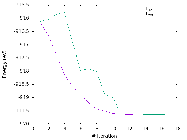
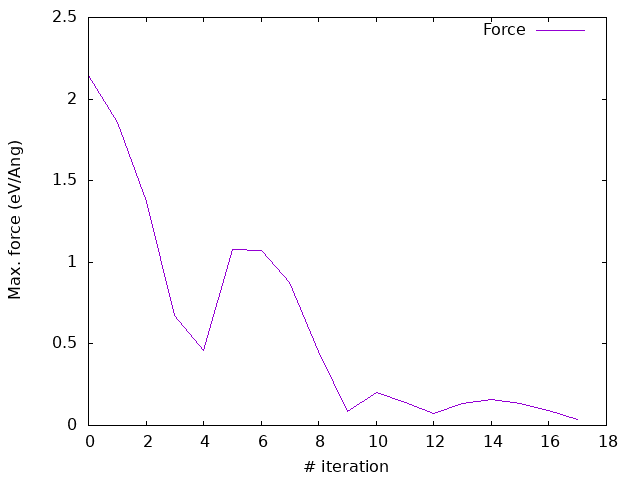
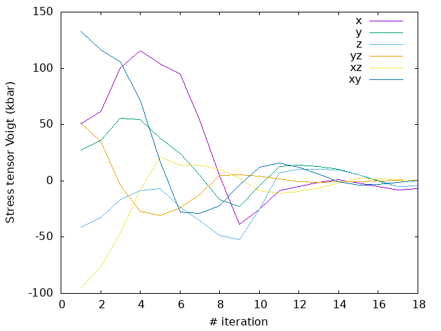
As you can see, now the forces converges quite nicely, with a monotonic decrease in the energy and a cleaner evolution of the stress (even if not entirely monotonic).

This method is always quite robust, and particularly efficient in the case of variable-cell. It can be generally counted on to bring systems closer to the optimal structure, and the final relaxation can be done afterwards with a faster method. We can even start with some extra kinetic energy, in the form of some ‘starting temperature’, to wiggle things around and free the system from any undesired local minimum.